Cluster-mass for EEG data
We will see and apply in R the permutation-based
cluster-mass method proposed by Maris and
Oostenveld, 2007 and developed in the R package
permuco4brain by Frossard
and Renaud, 2018, using electroencephalography (EEG) data. The
cluster-mass is computed considering the following scenarios:
- the time series of one channel: temporal cluster-mass;
- the time series of multiple channels: spatial-temporal cluster-mass.
Finally, the All-Resolution Inference (ARI) from Rosenblatt et
al. 2018 is applied to compute the lower bound for the true
discovery proportion (TDP) for the clusters found by the methods cited
above. We will use the ARIeeg and hommel
R packages here.
Packages
First of all, you need to install and load the following packages:
rm(list = ls())
#remotes::install_github("angeella/ARIeeg")
#remotes::install_github("jaromilfrossard/permuco4brain")
#remotes::install_github("jaromilfrossard/permuco")
#library(ARIeeg) #to compute ARI for spatial-temporal clusters
library(permuco4brain) #to compute the spatial-temporal clusters
library(plotly) # to create interactive plots (optional)
library(tidyverse) #collection of R packages (e.g., ggplot2, dplyr)
library(permuco) #to compute the temporal clusters
library(hommel) #to compute ARI for temporal clustersData
We analyze the dataset from the ARIeeg package which is
an Event-Related Potential (ERP) experiment composed
of:
- 20 Subjects;
- 32 Channels;
- Stimuli: pictures of
- (f): fear face;
- (h): happiness face;
- (d): disgusted face;
- (n): neutral face;
- (o): object.
\(500\) time points of brain signals are recorded for each subject and stimuli.
You can load the data using the following command:
Let’s see how the structure of the dataset:
## List of 7
## $ signals : tibble [50,000 × 32] (S3: tbl_df/tbl/data.frame)
## ..$ Fp1 : num [1:50000] -3.8308 -1.6821 -0.0565 -0.1089 -0.1812 ...
## ..$ Fp2 : num [1:50000] -5.709 -3.068 -0.912 -0.993 -1.056 ...
## ..$ F3 : num [1:50000] 0.45 0.872 1.176 1.109 1.04 ...
## ..$ F4 : num [1:50000] -0.85658 -0.30835 0.13854 0.06447 0.00742 ...
## ..$ F7 : num [1:50000] 0.583 0.71 0.737 0.739 0.771 ...
## ..$ F8 : num [1:50000] -1.466 -1.156 -0.87 -0.804 -0.707 ...
## ..$ FC1 : num [1:50000] 1.82 1.84 1.94 1.9 1.86 ...
## ..$ FC2 : num [1:50000] 0.707 0.785 0.915 0.857 0.817 ...
## ..$ C3 : num [1:50000] 2.08 1.92 1.83 1.82 1.78 ...
## ..$ C4 : num [1:50000] -0.41 -0.394 -0.27 -0.229 -0.167 ...
## ..$ T7 : num [1:50000] 1.98 1.5 1 1.19 1.33 ...
## ..$ T8 : num [1:50000] -0.978 -1.277 -1.476 -1.33 -1.174 ...
## ..$ CP1 : num [1:50000] 0.686 0.574 0.535 0.516 0.497 ...
## ..$ CP2 : num [1:50000] -0.408 -0.383 -0.284 -0.26 -0.23 ...
## ..$ P7 : num [1:50000] 2.184 1.374 0.622 0.535 0.436 ...
## ..$ P8 : num [1:50000] -1.12 -1.39 -1.65 -1.56 -1.48 ...
## ..$ P3 : num [1:50000] 1.148 0.882 0.671 0.631 0.584 ...
## ..$ P4 : num [1:50000] -1.59 -1.46 -1.28 -1.21 -1.14 ...
## ..$ PO7 : num [1:50000] 1.113 0.479 -0.116 -0.148 -0.195 ...
## ..$ PO8 : num [1:50000] -1.18 -1.36 -1.51 -1.48 -1.47 ...
## ..$ O1 : num [1:50000] 0.187 -0.255 -0.695 -0.698 -0.725 ...
## ..$ O2 : num [1:50000] -0.376 -0.694 -1 -0.994 -1.014 ...
## ..$ Fz : num [1:50000] 0.491 0.815 1.116 1.038 0.977 ...
## ..$ FCz : num [1:50000] 1.65 1.67 1.78 1.71 1.67 ...
## ..$ Cz : num [1:50000] 1.021 0.977 1.026 0.966 0.917 ...
## ..$ CPz : num [1:50000] 0.085 0.0765 0.1379 0.1341 0.136 ...
## ..$ Pz : num [1:50000] -0.264 -0.277 -0.233 -0.206 -0.176 ...
## ..$ RM : num [1:50000] -0.232 -1.237 -2.129 -2.064 -1.947 ...
## ..$ EOGvo: num [1:50000] -0.0194 -0.1595 -0.2224 -0.2223 -0.1851 ...
## ..$ EOGvu: num [1:50000] -2.85 -2.77 -2.66 -2.54 -2.44 ...
## ..$ EOGhl: num [1:50000] 3.025 1.769 0.735 0.625 0.508 ...
## ..$ EOGhr: num [1:50000] -1.16 -1.34 -1.59 -1.54 -1.47 ...
## $ srate : num 500
## $ events : tibble [100 × 6] (S3: tbl_df/tbl/data.frame)
## ..$ event_onset: num [1:100] 101 601 1101 1601 2101 ...
## ..$ event_time : num [1:100] 0.2 0.2 0.2 0.2 0.2 0.2 0.2 0.2 0.2 0.2 ...
## ..$ event_type : num [1:100] 1 2 3 4 5 1 2 3 4 5 ...
## ..$ epoch : num [1:100] 1 2 3 4 5 6 7 8 9 10 ...
## ..$ time : num [1:100] 0 0 0 0 0 0 0 0 0 0 ...
## ..$ subj : num [1:100] 1 1 1 1 1 2 2 2 2 2 ...
## $ chan_info: tibble [32 × 9] (S3: tbl_df/tbl/data.frame)
## ..$ electrode: chr [1:32] "Fp1" "Fp2" "F3" "F4" ...
## ..$ radius : num [1:32] 1 1 1 1 1 1 1 1 1 1 ...
## ..$ theta : num [1:32] -93 93 -62 62 -95 95 -33 33 -48 48 ...
## ..$ phi : num [1:32] -72 72 -50 50 -36 36 -45 45 0 0 ...
## ..$ cart_x : num [1:32] -26.1 26.1 -48.2 48.1 -68.4 ...
## ..$ cart_y : num [1:32] 80.8 80.8 57.6 57.6 49.9 ...
## ..$ cart_z : num [1:32] -4 -4 39.87 39.89 -7.49 ...
## ..$ x : num [1:32] -28.7 28.7 -39.9 39.9 -76.9 ...
## ..$ y : num [1:32] 88.5 88.5 47.5 47.5 55.8 ...
## $ timings : tibble [50,000 × 3] (S3: tbl_df/tbl/data.frame)
## ..$ time : num [1:50000] -0.2 -0.198 -0.196 -0.194 -0.192 -0.19 -0.188 -0.186 -0.184 -0.182 ...
## ..$ epoch : int [1:50000] 1 1 1 1 1 1 1 1 1 1 ...
## ..$ sample: int [1:50000] 1 2 3 4 5 6 7 8 9 10 ...
## $ reference: NULL
## $ epochs : epoch_nf [100 × 3] (S3: epoch_info/tbl_df/tbl/data.frame)
## ..$ epoch : int [1:100] 1 2 3 4 5 6 7 8 9 10 ...
## ..$ participant_id: chr [1:100] "ae011s" "ae012s" "ae013s" "ae014s" ...
## ..$ recording : chr [1:100] "ae011s" "ae012s" "ae013s" "ae014s" ...
## - attr(*, "class")= chr [1:2] "eeg_epochs" "eeg_data"It is a list (eeg_data class object from
eegUtils package) composed of 7 objects (the
reference one is NULL). The
eegUtils package permits to preprocess and plot EEG data.
More information here.
So, we have:
signals:tibbleobject, i.e., data frame composed by \(50000\) observations (brain signals across \(500\) time points for \(100 = 5 \times 20\) stimulus-subject combinations) and \(32\) variables (channels);srate: a single numeric value giving the sampling rate of the data in Hz. In this case, the signal includes \(500\) different time points;events:tibbleobject composed of \(100\) observations, i.e., experiment design (\(5\) stimuli for each subject, \(100 = 5 \times 20\)) and \(6\) variables (event onset in samples, events time in seconds, id stimulus, epoch, id time, id subject);chan_info:tibbleobject composed by \(32\) observations (channels) and \(9\) variables (name of electrode, Cartesian 3D coordinates etc);timings:tibbleobject containing a description of each row in time (s) and sample numbers (samples). We have in this case \(50000 = 100 \times 500\) rows, \(100 = 5 \times 20\) epochs (one for each combination stimuli-subjects), \(500\) different time points;epoch: containing information about the data epochs (not relevant for this analysis).
EDA
We drop off the final five bad channels (electrode locations are missing) and select two conditions, i.e., disgust face (number \(3\)) and object (number \(5\)):
m <- nrow(dati$chan_info)
chans <- dati$chan_info$electrode[c(1:(m-5))]
dati <-
dati %>%
eegUtils::select_elecs(chans)%>%
eegUtils::select_epochs(epoch_events = c(3,5))Let’s plot the global mean of the signal under the two selected conditions in the channels Fp1, Fp2, F3, and F4.
The observations in signals are stacked considering the
following structure (first subject, then stimuli, then time):
| SUBJECT | STIMULI | TIME |
|---|---|---|
| 1 | 3 | 1 |
| 2 | 3 | 2 |
| 3 | 3 | 3 |
| 4 | 3 | 4 |
| 5 | 3 | 5 |
| 6 | 3 | 6 |
chans <- c("Fp1", "Fp2", "F3", "F4")
dati_sel <- dati %>%
eegUtils::select_elecs(chans)
dati_sel$signals$subj <- rep(seq(20), 500*2)
dati_sel$signals$condition <- rep(c("3","5"), each = 500*20)
dati_sel$signals$time <- rep(seq(500), 20*2)
A<-dati_sel$signals %>%
pivot_longer(cols = all_of(chans)) %>%
ggplot(aes(x = time, y = value)) +
geom_line(aes(group = condition)) +
stat_summary(
fun = "mean", geom = "line", alpha = 1, linewidth = 1,
aes(color = condition),show.legend = TRUE
) +
geom_vline(xintercept = 0, linetype = "dashed") +
geom_vline(xintercept = .17, linetype = "dotted") +
theme(legend.position = "bottom")+
scale_color_manual(labels = c("Disgust", "Object"),
values = c("#80bfff", "#ff8080"))+
facet_wrap(~name)
A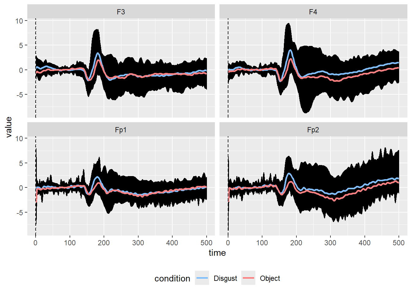
if you want an interactive plot, you can use the function
ggplotly from the package plotly:
Theory
Multiple testing problem?
The aim is to test if the difference in brain signal during the two conditions differs from \(0\) for each time point, i.e., \(500\). If the complete set of channels is considered, we also have tests for each channel, i.e., \(27\), returning a total number of tests equals \(500 \cdot 27\). Therefore, we have \(500\) or \(500 \cdot 27\) statistical tests to perform at group-level, so considering the random subject effect.
We must deal with multiple statistical tests, and standard family-wise error rate (FWER) correction methods such as Bonferroni do not capture the time(-spatial) correlation structure of the statistical tests; it will be a conservative method.
The cluster mass method proposed by Maris and Oostenveld, 2007 is then used. It is based on permutation theory; it gains some power with respect to other procedures correcting at the (spatial-)temporal cluster level instead of at the level of single tests.
It is similar to the cluster mass approach in the fMRI framework, but in this case, the voxels, i.e., the single object of the analysis, are expressed in terms of time points or combination time points/channels. The method can then gain some power with respect to some traditional conservative FWER correction methods exploiting the (spatial-)temporal structure of the data.
So, let’s see how to compute the statistical tests.
Repeated Measures ANOVA Model
The cluster mass method is based on the repeated measures ANOVA model, i.e.,
\[ \boxed{y = \mathbf{1} \mu + X_{\eta} \eta + X_{\pi}\pi + X_{\gamma}\gamma + \epsilon} \]
where \(\mathbf{1}\) is a matrix of ones having dimensions \(N \times 1\) and
\(y \in \mathbb{R}^{N \times 1}\) is the response variables, i.e., the signal, in our case \(N = n_{\text{subj}} \times n_{\text{stimuli}} = 40\);
\(\mu\) is the intercept;
\(X_{\eta} \in \mathbb{R}^{N \times n_{\text{stimuli}}}\) is the design matrix describing the fixed effect regarding the stimuli, and \(\eta \in \mathbb{R}^{n_{\text{stimuli}} \times 1}\) the corresponding parameter of interest;
\(X_{\pi} \in \mathbb{R}^{N \times n_{\text{subj}}}\) is the design matrix describing the random effect regarding the subjects, and \(\pi \in \mathbb{R}^{n_{\text{subj}} \times 1}\) the corresponding subject effect.
\(X_{\gamma} \in \mathbb{R}^{N \times (n_{\text{subj}} n_{\text{stimuli}})}\) is the design matrix describing the interaction effects between subjects and conditions, and \(\gamma \in \mathbb{R}^{(n_{\text{subj}} n_{\text{stimuli}}) \times 1}\) the corresponding interaction effect;
\(\epsilon \in \mathbb{R}^{N \times 1}\) is the error term with \(0\) mean and variance \(\sigma^2 I_N\).
Therefore, \(y \sim (1\mu + X_{\eta} \eta, \Sigma)\), \(\pi \sim (0, \Sigma_{\pi})\) and \(\gamma \sim (0,\Sigma_{\gamma})\). Generally, \(\Sigma_{\pi} = \sigma^2_{\pi} I_{n_{subj}}\) and the sigma-restriction constraints are assumed.
We want to make inference on \(\eta\), such that \(H_0: \eta = 0\) vs \(H_1: \eta \ne 0\). We do that using the F statistic, i.e.,
\[ F = \dfrac{y^\top H_{X_{\eta}} y / (n_{\text{stimuli}} - 1)}{ y^\top H_{X_{\gamma}}y/(n_{\text{stimuli}} -1)(n_{\text{subj}} -1)} \] where \(H_{X}\) is the projection matrix of \(X\), i.e., \(H_{X} = X(X^\top X)^{-1} X^\top\). In order to compute this test, we use an alternative definition of \(F\) based on the residuals:
\[ F_r = \dfrac{r^\top H_{X_{\eta}} r / (n_{\text{stimuli}} - 1)}{ r^\top H_{X_{\gamma}}r/(n_{\text{stimuli}} -1)(n_{\text{subj}} -1)} \]
where \(r = (H_{X_{\eta}} + H_{X_{\gamma}})y\). For further details, see Kherad Pajouh and Renaud, 2014.
So, let the group of permutation, including the identity transformation, \(\mathcal{P}\), we use \(r^\star = P r\), where \(P \in \mathcal{P}\) to compute the null distribution of our test, i.e., \(\mathcal{R}\), and then the \(p\)-value, i.e.,
\[ \text{$p$-value} = \dfrac{1}{B} \sum_{F^\star_r \in \mathcal{R}} \mathbb{I}(|F^\star_r| \ge |F_r|) \]
if the two-tailed is considered, where \(F^\star_r = f(r^\star)\).
We have this model for each time point \(t \in \{1, \dots, 500\}\) and each channel, so finally we will have \(n_{\text{time-points}} \times n_{\text{channels}}\) statistical tests/\(p\)-values (raw).
Temporal Cluster mass
This method has been proposed by Maris and Oostenveld, 2007. It assumes that an effect will appear in clusters of adjacent time frames. Having statistics for each time point, we form these clusters using a threshold \(\tau\) as follows:

All contiguous time points with statistics above this threshold define a single cluster \(C_i\) with \(i \in \{1, \dots, n_C\}\), where \(n_C\) is the number of clusters found.
For each time point in the same cluster \(C_i\), we assign the same cluster mass statistic \(m_i = f(C_i)\), where \(f\) is the function that summarizes the statistics of the entire cluster.
Typically, it is the sum of the \(F\) statistics. The null distribution of the cluster mass \(\mathcal{M}\) is computed by iterating the above process for each permutation.
The contribution of a permutation to the cluster-mass null distribution is the maximum overall cluster masses of that permutation. So for each \(P \in \mathcal{P}\):
- compute the \(t\) permuted statistics
- Find the \(n_C^\star\) clusters \(C_i^\star\) considering the same threshold \(\tau\)
- Compute \(m_i^\star = f(C_i^\star)\)
- Find the maximum over \(i = \{1, \dots, n_C^\star\}\)
To check the significance of the cluster \(C_i\) of interest, we compare the observed cluster mass \(m_i = f(C_i)\) with the cluster mass null distribution \(\mathcal{M}\). Therefore, for each cluster \(C_i\), we have the associated \(p\)-values computed as
\[ p_i = \dfrac{1}{n_P} \sum_{m^\star \in \mathcal{M}} I\{m^\star \ge m_i\} \]
where \(m^\star \in \mathcal{M}\) is then calculated given permutation statistics.
This method makes sense when analyzing EEG data because if a difference in brain activity is thought to occur at time \(s\) for a given factor, then it is very likely that this difference will also occur at time \(s + 1\) (or \(s - 1\)).
Spatial-temporal Cluster mass
In this case, we use graph theory, where the vertices represent the channels and the edges represent the adjacency relationships between two channels.
The adjacency must be defined using prior information, so the three-dimensional Euclidean distance between channels is used. Two channels are defined as adjacent if their Euclidean distance is less than the threshold \(\delta\), where \(\delta\) is the smallest Euclidean distance that yields a connected graph Cheval, et al., 2018).
This follows from the fact that there is no unconnected subgraph for a connected graph. The existence of subgraphs implies that some tests cannot be entered in the same cluster, which is not a reasonable assumption for the present analysis (Frossard and Renaud, 2018; Frossard, 2019).
Once we have a definition of spatial contiguity, we need to define temporal contiguity. We reproduce this graph \(n_{\text{time-points}}\) times, and we have edges between pairs of two vertices associated with the same electrode if they are temporally adjacent.
The final graph has a total number of vertices, i.e., the number of tests, equals (\(n_{\text{channels}} \times n_{\text{time-points}}\)). The following figure shows an example with \(64\) channels and \(3\) time measures:

We compute for each spatial-temporal cluster the cluster-mass statistic as before. We then delete all the vertices in which statistics are below a threshold, e.g., the \(95\) percentile of the null distribution of the \(F\) statistics. So, we have a new graph composed of multiple connected components, where each connected component defines the spatial-temporal cluster.
The cluster-mass null distribution is calculated using permutations that preserve the spatial-temporal correlation structure of the statistical tests, i.e., no changing the position of the electrodes and mixing the time points.
We will construct a three-dimensional array, where the first dimension represents the design of our experiments (subjects of \(\times\) stimuli), the second one the time points, and the third one the electrodes.
So, we apply permutations only in the first dimension using the method proposed by Kherad Pajouh and Renaud, 2014.
Application
In R, all of this is possible thanks to the
permuco and permuco4brain packages developed
by Frossard
and Renaud, 2018.
Temporal Cluster-Mass
So, we select one channel from our dataset, e.g., the Fp1:
- Construct the \(y\). We need to construct the two-dimensional signal matrix, having dimensions \(40 \times 500\):
Fp1<-dati %>%
eegUtils::select_elecs("Fp1")%>%
eegUtils::select_epochs(epoch_events = c(3,5))
signal_Fp1 <- matrix(Fp1$signals$Fp1,
nrow = 40,
byrow = TRUE) #remember the structure of the signals tibble
dim(signal_Fp1)## [1] 40 500So, signal_Fp1 is a data frame that expresses the
signals recorded in the Fp1 channel under the two
conditions across \(500\) time points
for \(20\) subjects.
- Construct the matrix containing the covariates information (i.e., subject and conditions), having dimensions \(40 \times 2\):
design <-
data.frame(participant_id =rep(seq(20), 2),
condition =rep(c(3,5), 20)) #as in Fp1
dim(design)## [1] 40 2- Define the repeated measures ANOVA formula:
In the formula, we need to specify the Error(.) term
since we are dealing with a repeated measures design. We specify a
subject-level random effect and a condition fixed effect nested within
subjects.
Thanks to the permuco package, we can apply the temporal
cluster-mass for the channel Fp1:
## Effect: condition.
## Alternative Hypothesis: two.sided.
## Statistic: fisher(1, 18).
## Resampling Method: Rd_kheradPajouh_renaud.
## Type of Resampling: permutation.
## Number of Dependant Variables: 500.
## Number of Resamples: 5000.
## Multiple Comparisons Procedure: clustermass.
## Threshold: 4.413873.
## Mass Function: the sum.
## Table of clusters.
##
## start end cluster mass P(>mass)
## 1 115 116 10.80609 0.8658
## 2 167 212 549.21173 0.0230
## 3 216 225 73.28732 0.2668
## 4 316 318 15.30207 0.8272
## 5 364 366 14.74535 0.8382
## 6 378 382 31.66024 0.6028Here we can see:
The threshold used to construct the temporal clusters, i.e., 4.4138734 (\(0.95\) quantile of the test statistic);
The type of cluster mass function, i.e., the sum of single statistical tests time contiguous;
When the cluster starts and ends, the value of the cluster mass and the associated corrected \(p\)-values.
For example, considering the significant cluster (i.e., 2), we can compute the cluster mass as:
## [1] 549.2117We can also plot the temporal clusters:
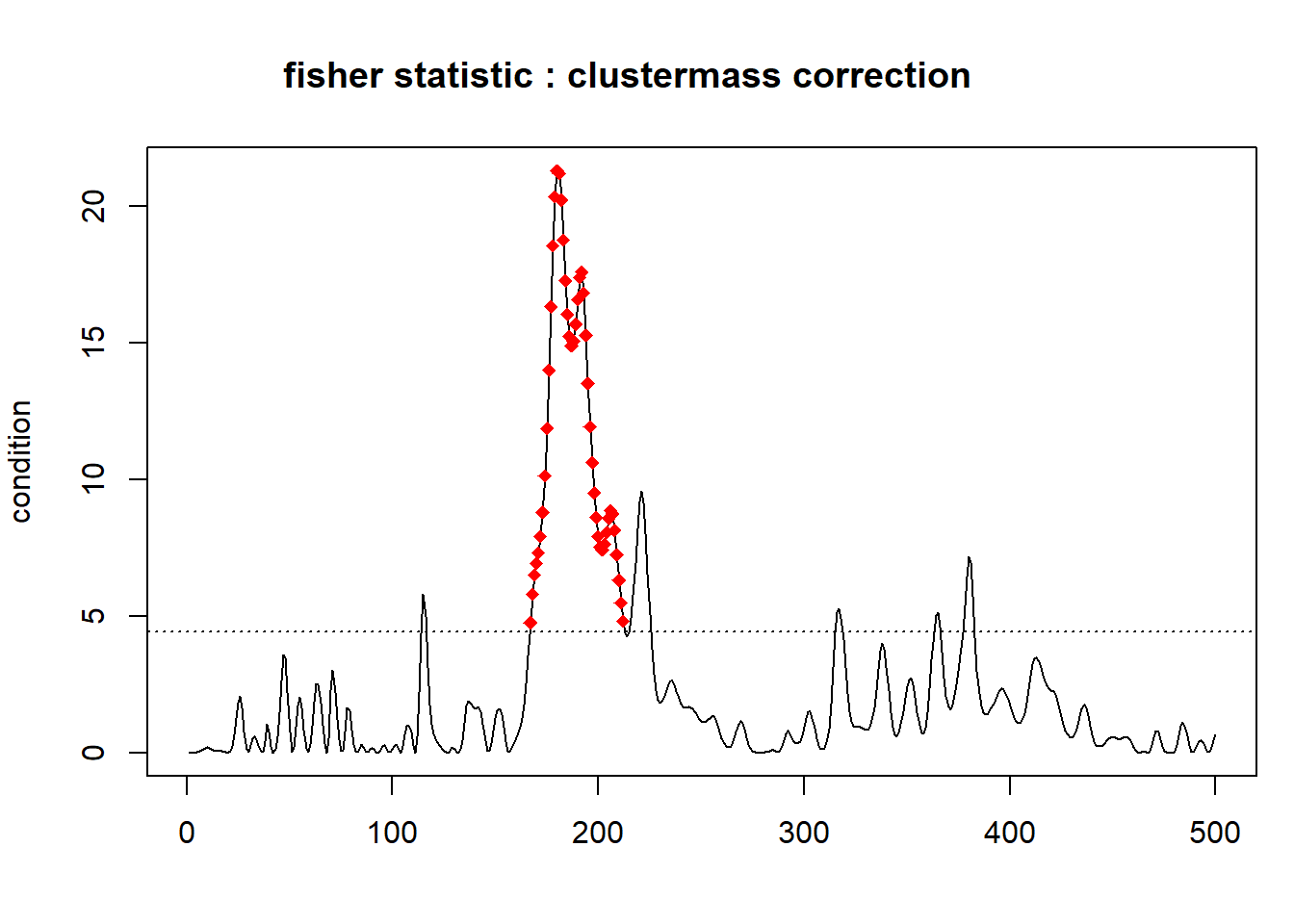
The red dots represent the significant temporal cluster for the channel Fp1 composed of the time points from \(167\) to \(212\) using a threshold equal to 4.4138734.
ARI in EEG cluster mass
However, our significant cluster says only that at least one test is different from \(0\), we don’t know how many tests/time-points are significant (spatial specificity paradox).
So, we can apply ARI to understand the lower bound of the number of true discovery proportions. The cluster comprises the time points from \(167\) to \(212\), i.e., the cluster size equals \(46\).
praw <- lm_Fp1$multiple_comparison$condition$uncorrected$main[,2] #extract raw pvalues
output_lm <- summary(lm_Fp1)$condition
TDP <- sapply(seq(nrow(output_lm)), function(x){
ix <- c(output_lm$start[x]:output_lm$end[x]) #set of indices hyp of interest
round(discoveries(hommel(praw), ix = ix)/length(ix),3) #apply parametric ARI
}
)
data.frame(clustermass = output_lm$`cluster mass`,
pmass = output_lm$`P(>mass)`,
TDP = TDP)## clustermass pmass TDP
## 1 10.80609 0.8658 0.000
## 2 549.21173 0.0230 0.174
## 3 73.28732 0.2668 0.000
## 4 15.30207 0.8272 0.000
## 5 14.74535 0.8382 0.000
## 6 31.66024 0.6028 0.000Therefore, the second cluster has at least 17.4\(\%\) true active time points.
Spatial-Temporal Cluster-Mass
- Construct the \(y\). We need to construct the three-dimensional signal array, having dimensions \(40 \times 500 \times 27\):
signal <- array(NA, dim = c(40,500, 27))
chn <- eegUtils::channel_names(dati)[1:27]
for(i in seq(27)){
chn_utils<-dati %>%
eegUtils::select_elecs(chn[i])%>%
eegUtils::select_epochs(epoch_events = c(3,5))
signal[,,i] <- matrix(as.data.frame(chn_utils$signals)[,1],
nrow = 40,
byrow = TRUE)
}
dimnames(signal) <- list(NULL, NULL, chn)- Construct as before the matrix containing the covariates information having dimensions \(40 \times 2\):
design <-
data.frame(participant_id =rep(seq(20), 2),
condition =rep(c(3,5), 20)) #as before
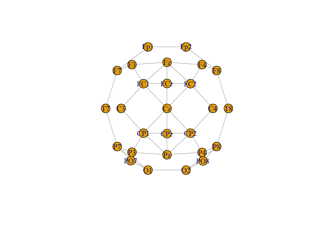
dim(design)## [1] 40 2- Construct the graph, using \(\delta = 53mm\) (the maximal distance for
adjacency of two channels) and the function
position_to_graphfrom thepermuco4brainpackage:
graph <- position_to_graph(as.data.frame(dati$chan_info)[c(1:27),],
name = "electrode",
delta = 53,
x = "cart_x",
y = "cart_y",
z = "cart_z")
graph## IGRAPH 9685357 UN-- 27 48 --
## + attr: name (v/c), x (v/n), y (v/n), z (v/n)
## + edges from 9685357 (vertex names):
## [1] Fp1--Fp2 Fp1--F7 Fp2--F8 F3 --F7 F3 --FC1 F3 --Fz F4 --F8 F4 --FC2
## [9] F4 --Fz F7 --T7 F8 --T8 FC1--C3 FC1--Fz FC1--FCz FC1--Cz FC2--C4
## [17] FC2--Fz FC2--FCz FC2--Cz C3 --CP1 C4 --CP2 T7 --P7 T8 --P8 CP1--P3
## [25] CP1--Cz CP1--CPz CP1--Pz CP2--P4 CP2--Cz CP2--CPz CP2--Pz P7 --P3
## [33] P7 --PO7 P7 --O1 P8 --P4 P8 --PO8 P8 --O2 P3 --PO7 P3 --Pz P4 --PO8
## [41] P4 --Pz PO7--O1 PO8--O2 O1 --O2 Fz --FCz FCz--Cz Cz --CPz CPz--PzThe object graph is an igraph object that
computes the channels’ adjacency matrix. You can see two letters
UN-- that stand for unweighted undirected named graph. The
graph comprises \(27\) nodes (i.e.,
channels) and \(48\) edges.
How do you choose \(delta\)? I
simply increased the value of \(delta\)
until the position_to_graph function returns the following
warning:
Warning: This graph has more than 1 cluster. It is not valid for a clustermass test. Check the position of the channels or increase delta.
- Define the repeated measures ANOVA formula:
Finally, run the main function:
model <- permuco4brain::brainperm(formula = f,
data = design,
graph = graph,
np = 1000,
multcomp = "clustermass",
return_distribution = TRUE)## Computing Effect:
## 1 (condition) of 1. Start at 2026-07-06 11:32:21.509352.## Warning: package 'future' was built under R version 4.4.3where np indicates the number of permutation.
Then, we can analyze the output:
## Effect: condition.
## Alternative Hypothesis: two.sided.
## Statistic: fisher(1, 18).
## Resampling Method: Rd_kheradPajouh_renaud.
## Type of Resampling: permutation.
## Number of Dependant Variables: 13500.
## Number of Resamples: 1000.
## Multiple Comparisons Procedure: clustermass.
## Threshold: 4.413873.
## Mass Function: the sum.
## Table of clusters.
##
## Cluster id First sample Last sample N. chan. Main chan. Main chan. length
## 1 1 42 43 1 T7 2
## 2 2 64 66 1 Fp2 3
## 3 3 64 66 1 P3 3
## 4 4 73 73 1 T8 1
## 5 5 73 73 1 P4 1
## 6 6 80 81 1 T8 2
## 7 7 83 88 1 T7 6
## 8 8 97 100 1 F3 4
## 9 9 112 114 1 C3 3
## 10 10 115 116 1 Fp1 2
## 11 11 162 250 25 Fp1 56
## 12 12 211 229 1 P7 19
## 13 13 217 223 2 Fz 7
## 14 14 233 237 1 P8 5
## 15 15 244 487 3 P8 244
## 16 16 262 349 8 CPz 81
## 17 17 291 500 8 P7 199
## 18 18 316 318 1 Fp1 3
## 19 19 354 360 2 CPz 5
## 20 20 364 366 1 Fp1 3
## 21 21 368 378 4 CP2 11
## 22 22 378 382 1 Fp1 5
## 23 23 497 499 1 P8 3
## N. test Clustermass P(>mass)
## 1 2 10.192298 1.000
## 2 3 14.229994 1.000
## 3 3 15.887277 1.000
## 4 1 4.995142 1.000
## 5 1 4.482731 1.000
## 6 2 9.948122 1.000
## 7 6 37.730924 0.999
## 8 4 22.040027 1.000
## 9 3 14.179013 1.000
## 10 2 10.806087 1.000
## 11 750 13639.972730 0.001
## 12 19 100.198542 0.976
## 13 9 42.025353 0.999
## 14 5 22.607432 0.999
## 15 309 3896.903241 0.089
## 16 330 2081.663209 0.250
## 17 774 7024.282254 0.022
## 18 3 15.302073 1.000
## 19 9 41.151044 0.999
## 20 3 14.745346 1.000
## 21 29 154.893529 0.949
## 22 5 31.660245 0.999
## 23 3 13.511188 1.000We have only two significant clusters. The first comprises \(25\) channels while the second is \(8\) channels, with main channels P7. You can see in detail the components of this cluster in
cls17 <- names(model$multiple_comparison$condition$clustermass$cluster$membership[which(as.vector(model$multiple_comparison$condition$clustermass$cluster$membership)==17)])
head(cls17,n = 10)## [1] "P7_291" "P7_292" "P7_293" "P7_294" "P7_295" "P7_296" "P7_297"
## [8] "P7_298" "PO7_298" "P7_299"You can see the significant cluster (in red) at fixed time points (e.g. 300) using plot:
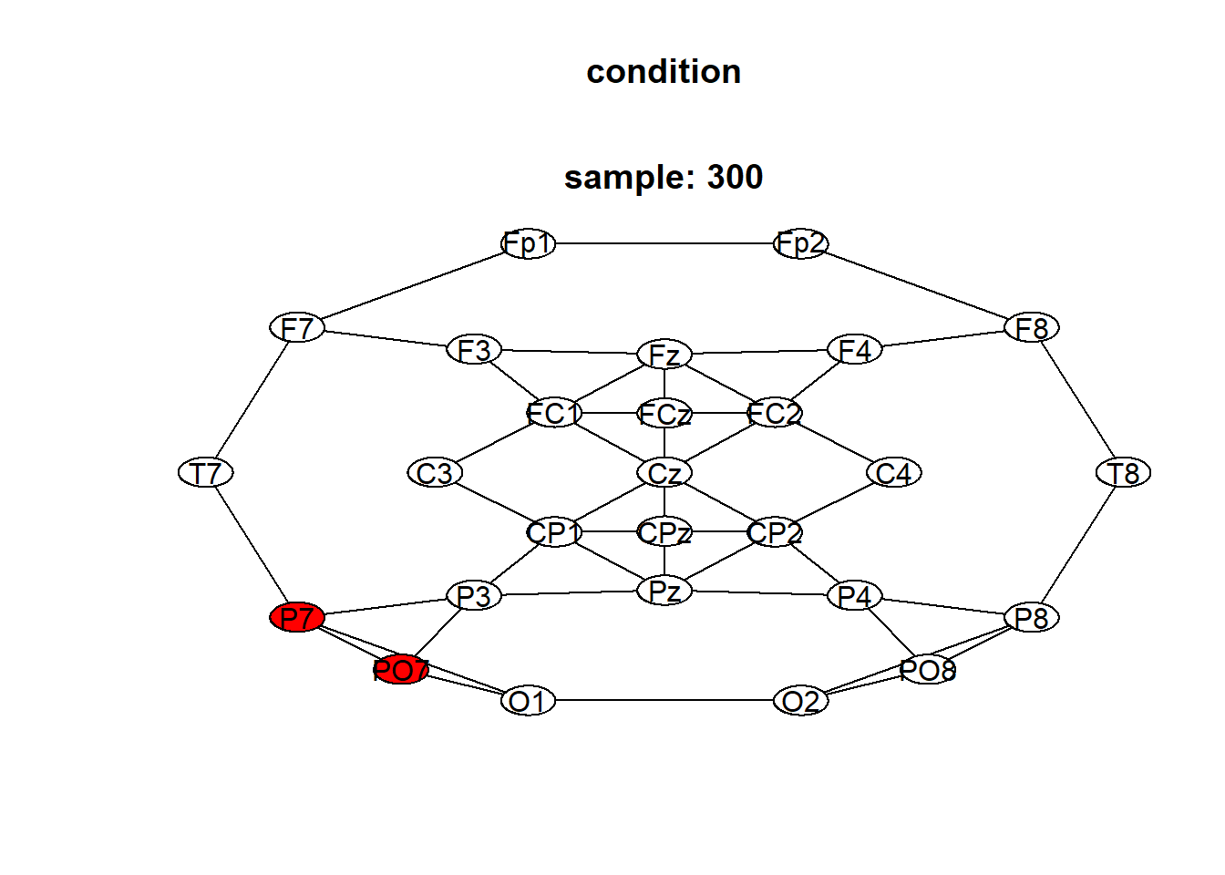
in fact:
## [1] "P7_300" "PO7_300"and the significant cluster over time and over channels using:
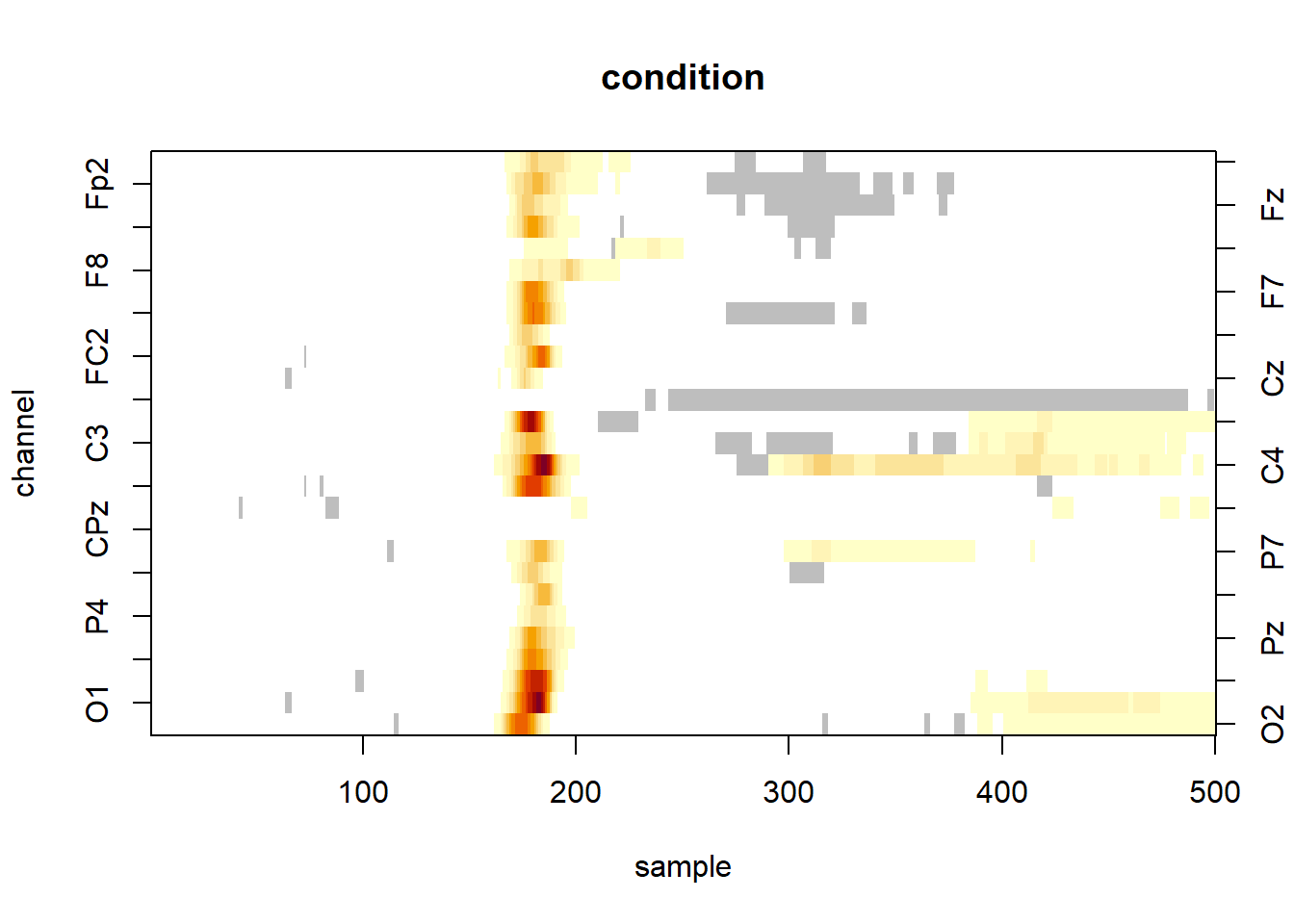
where the significant clusters are represented in a colour-scale (as a function of the individual statistics) and the non-significant one in grey. The white pixels are tests which statistic are below the threshold.
ARI in EEG spatial-temporal cluster analysis
However, our significant clusters say again that at least one combination channels/time-points is different from \(0\) as before, we do not know how many combinations are significant (spatial specificity paradox).
So, we can apply ARI to understand the lower bound of the number of true discovery proportion:
In this case, the lower bound for TDP equals \(0\) for all clusters, also if we consider the significant spatial-temporal clusters.
Why is that?
ARI is based on the Simes inequality to construct the critical vector that computes the lower bound for the TDP for the set \(S\) of hypotheses (i.e., \(\bar{a}(S)\)).
Therefore, the approach can be conservative under strong positive dependence among tests \(\rightarrow\) permutation-based ARI (Andreella et al. 2023).
Recalling the definition of \(\bar{a}\):
\[\bar{a}(S) = \max_{1 \le u \le |S|} 1 - u + |\{i \in S, p_i \le l_u\}|\]
where \(S\) is the set of hypothesis of interest (i.e., cluster), \(p_i\) is the raw p-values and \(l_i\) a suitable vector such that
\[\Pr(\cap_{i = 1}^{|N|} \{q_{(i)} \ge l_i\}) \le 1-\alpha\]
where \(N\) is the unknown set of inactive time-points/channels and \(q_{(i)}\) are their sorted \(p\)-values. In other words, the curve of the sorted \(p\)-values corresponding to inactive time-points/channels should lie completely above the \(l_i\) with probability at least \(1 − \alpha\).
paramteric ARI uses \(l_i = \dfrac{i \alpha}{m}\), where \(m\) is the total number of statistical tests.
To gain power in case of dependence between tests, we can consider \(l_i = \dfrac{i \lambda_{\alpha}}{m}\) and calibrate \(\lambda_{\alpha}\) using the \(p\)-values permutation null distribution such that \(l_i\) cuts the \(p\)-values null distribution to have the \(\alpha \%\) \(p\)-values distribution below it (i.e., it is a proper critical vector).
alpha <- 0.3
Test <- model$multiple_comparison$condition$uncorrected$distribution
dim(Test) <- c(dim(Test)[1], dim(Test)[2]*dim(Test)[3])
pv <- matrixStats::colRanks(-abs(Test)) / nrow(Test)## Warning in tiesMethodMissing(): [matrixStats (>= 1.3.0)] Please explicitly
## specify argument 'ties.method' when calling colRanks() and rowRanks() of
## matrixStats. This is because the current default ties.method="max" will
## eventually be updated to ties.method="average" in order to align with the
## default of base::rank(). If you are an end-user that cannot update the R code
## causing this, see ?matrixStats::matrixStats.options for how to temporarily
## disable this checklambda <- pARI::lambdaOpt(pvalues = pv,
family = "simes",
alpha = 0.3) #compute lambda
cvOpt = pARI::criticalVector(pvalues = pv,
family = "simes",
lambda = lambda,
alpha = 0.3) #compute l_i
plot(sort(pv[,1]), type = "l")
for(i in seq(ncol(pv))){
lines(sort(pv[,i])) #plot null distribution
}
lines(sort(pv[,1]), col = "red") #plot observed sorted p-values
lines(cvOpt, col = "blue") #plot l_i pARI
lines((c(1:nrow(pv))*alpha)/nrow(pv), col = "green") #plot l_i ARI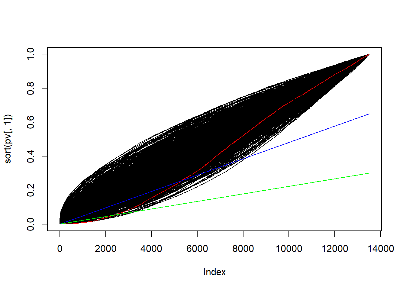
Since \(\lambda_{\alpha} > \alpha\) the permutation approach will outperfom ARI:
References
Maris, E., & Oostenveld, R. (2007). Nonparametric statistical testing of EEG-and MEG-data. Journal of neuroscience methods, 164(1), 177-190.
Kherad-Pajouh, S., & Renaud, O. (2015). A general permutation approach for analyzing repeated measures ANOVA and mixed-model designs. Statistical Papers, 56(4), 947-967.
Frossard, J. (2019). Permutation tests and multiple comparisons in the linear models and mixed linear models, with extension to experiments using electroencephalography. DOI: 10.13097/archive-ouverte/unige:125617.
Frossard, J. & O. Renaud (2018). Permuco: Permutation Tests for Regression, (Repeated Measures) ANOVA/ANCOVA and Comparison of Signals. R Packages.
Cheval, Boris, et al. “Avoiding sedentary behaviors requires more cortical resources than avoiding physical activity: An EEG study.” Neuropsychologia 119 (2018): 68-80.
Rosenblatt JD, Finos L, Weeda WD, Solari A, Goeman JJ. All-Resolutions Inference for brain imaging. Neuroimage. 2018 Nov 1;181:786-796. doi: 10.1016/j.neuroimage.2018.07.060. Epub 2018 Jul 27. PMID: 30056198.
Andreella, A, Hemerik, J, Finos, L, Weeda, W, Goeman, J. Permutation-based true discovery proportions for functional magnetic resonance imaging cluster analysis. Statistics in Medicine. 2023; 1- 30. doi: 10.1002/sim.9725
https://jaromilfrossard.netlify.app/post/2018-08-06-full-scalp-cluster-mass-test-for-eeg/